One definition of a limit, in place of about 169

Three conditions

A way to say "eventually" without saying when

A filter on a set X is a collection of subsets of X, thought of as the sets that are "big enough" for whatever purpose is at hand. It has to satisfy three conditions.

1. The empty set is not in it

   Otherwise "big enough" would include nothing at all.

2. Anything bigger is also in it

   If A is big enough and A ⊆ B, then B is big enough.

3. Two of them overlap in one

   If A and B are both big enough, so is A ∩ B. This is what lets you combine two conditions, the way N = max{N₁, N₂} does in an epsilon proof.

Three that come up constantly

The neighbourhood filter at a point x: all sets containing an open interval around x. This is "sufficiently close".

The tail filter at +∞: all sets containing a ray. This is "sufficiently large".

The principal filter on a set A: everything containing A. On X = {1,2,3,4} with A = {3,4} that is four sets.

Try building one

Below is every subset of {1,2,3,4}. Switch some on and the panel checks the three conditions against your collection, and names the pair that breaks whichever one fails.

Sequences first

The same convergence, said with sets

Before the general definition, the special case. Take the collection of subsets of ℕ whose complement is finite — the cofinite, or Fréchet, filter.

A set is in it exactly when it contains a tail. That is the first lemma, and it is what makes this filter mean "sufficiently large".

def frechetFilter : Filter ℕ :=
  Filter.cofinite

lemma frechet_tail_lemma (A : Set ℕ) :
  A ∈ frechetFilter ↔ ∃ a : ℕ, Set.Ici a ⊆ A :=by
  have h1 : A ∈ frechetFilter ↔ A ∈ (Filter.atTop : Filter ℕ) := by
    simp [frechetFilter, Nat.cofinite_eq_atTop]
  have h2 : A ∈ (Filter.atTop : Filter ℕ) ↔ ∃ N, ∀ n ≥ N, n ∈ A :=by
    exact (Filter.mem_atTop_sets)
  have h3 : (∃ N, ∀ n ≥ N, n ∈ A) ↔ ∃ N, Set.Ici N ⊆ A := by
    exact Eq.to_iff rfl
  exact (h1.trans h2).trans h3

Now fix a sequence and a candidate limit, and for each ε collect the indices where the sequence is already within ε.

Convergence in the usual sense says exactly that every one of those sets is in the filter.

Nothing has been gained yet — this is the same statement twice. What it buys is the change of shape. The left side quantifies over indices; the right side asks whether a set is in a collection. The next section is where that pays.

lemma seq_filter_equiv
    (a : ℕ → ℝ) (L : ℝ) :
    (∀ ε > (0 : ℝ), ∃ N : ℕ, ∀ n ≥ N, |a n - L| < ε) ↔
    (∀ ε > (0 : ℝ), {n : ℕ | |a n - L| < ε} ∈ frechetFilter) :=by
  constructor
  · intro h ε hε
    rcases h ε hε with ⟨N, hN⟩
    have htail :
        ∃ N, Set.Ici N ⊆ {n : ℕ | |a n - L| < ε} := by
      refine ⟨N, ?_⟩
      intro n hn
      exact hN n hn
    exact (frechet_tail_lemma _).mpr htail
  ·
    intro h ε hε
    have h' :
    ∃ N, Set.Ici N ⊆ {n : ℕ | |a n - L| < ε} := by
      apply (frechet_tail_lemma _).mp
      exact h ε hε
    rcases h' with ⟨N, hN⟩
    refine ⟨N, ?_⟩
    intro n hn
    exact hN hn

The whole idea

Drop the specifics and the 169 collapse

Sequences used two particular filters: the tail filter on ℕ and the neighbourhood filter at L. Leave both unspecified and the definition stops being about sequences.

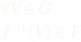
X and Y are sets, F is a filter on X, G is a filter on Y, and f maps X to Y. Read it as: whatever counts as big enough in the target, its preimage counts as big enough in the source.

Every cell of the grid in Section 01 is this statement with a particular F and G filled in. A one-sided limit is a different F. Running off to infinity is a different G. Sequences are a different X. The definition does not change.

One quantifier instead of three

The other thing worth noticing is the shape. The epsilon version alternates quantifiers: for all ε, there exists N, for all n. Alternating quantifiers are what make analysis proofs fiddly, because each one has to be introduced and discharged in the right order. The filter version has one.

Composition, which is where the saving shows up

Classically this is a lemma about points, and it has a version for every combination of ways the three limits can be taken.

With filters it is a statement about three filters and two functions, and the proof is to pull a set backwards twice.

Step through it. The set starts in the target and travels back to the source, one preimage at a time.

example {X Y Z : Type*} {F : Filter X} {G : Filter Y} {H : Filter Z}
    {f : X → Y} {g : Y → Z}
    (hf : Tendsto f F G) (hg : Tendsto g G H) :
    Tendsto (g ∘ f) F H := by
    refine (tendsto_def.mpr ?_)
    intro s hs
    have hf' := tendsto_def.mp hf
    have hg' := tendsto_def.mp hg
    have hG : g ⁻¹' s ∈ G := hg' s hs
    have hF : f ⁻¹' (g ⁻¹' s) ∈ F := hf' _ hG
    simpa [Set.preimage, Function.comp] using hF

theorem tendsto_const_seq (c : ℝ) :
    Tendsto (fun _ : ℕ => c) (atTop : Filter ℕ) (𝓝 c) := by
  refine (tendsto_def.mpr ?_)
  intro s hs
  have h': c∈s:=by
    exact mem_of_mem_nhds hs
  have hpre:(fun _ : ℕ => c)⁻¹'s=Set.univ :=by
    ext n
    simp[h']
  simp[hpre]

The same definition again

Continuity is not a new idea

Take the general definition, put the neighbourhood filter at x in the source slot and the neighbourhood filter at f(x) in the target slot. That is continuity at a point.

Points close enough to x land close enough to f(x). The sequential definition says the same thing along sequences, and the epsilon-delta definition says it with two explicit numbers.

The two agree, and in Lean that is one line, because Mathlib already carries the bridge between its topological and metric definitions.

-- ε–δ definition of continuity at a point x₀ for f : ℝ → ℝ
def cont_eps_delta (f : ℝ → ℝ) (x₀ : ℝ) : Prop :=
  ∀ ε > 0, ∃ δ > 0, ∀ {x : ℝ}, dist x x₀ < δ → dist (f x) (f x₀) < ε

theorem cont_filter_equiv (f : ℝ → ℝ) (x₀ : ℝ) :
  ContinuousAt f x₀ ↔ cont_eps_delta f x₀ := by
  simpa [cont_eps_delta] using
    (Metric.continuousAt_iff (f := f) : ContinuousAt f x₀ ↔ _)

A sum of continuous functions

Classically you pick N_f and N_g for the two functions and take the larger. With filters you build the pair (f, g) as a single map into ℝ × ℝ, observe that addition is continuous, and compose.

theorem continuousAt_add
    (f g : ℝ → ℝ) (x : ℝ)
    (hf : ContinuousAt f x)
    (hg : ContinuousAt g x) :
    ContinuousAt (fun y => f y + g y) x := by
  let h : ℝ → ℝ × ℝ := fun y => (f y, g y)
  let k : ℝ × ℝ → ℝ := fun p => p.1 + p.2
  have h_pair : ContinuousAt h x := by
    simpa [h] using hf.prodMk hg
  have h_add : ContinuousAt k (h x) := by
    have hk : Continuous k := by
      simpa [k] using
        (continuous_fst.add continuous_snd :
          Continuous fun p : ℝ × ℝ => p.1 + p.2)
    simpa [h] using hk.continuousAt (x := h x)
  have h_comp : ContinuousAt (fun y => k (h y)) x :=
    ContinuousAt.comp' (f := h) (g := k) (x := x) h_add h_pair
  simpa [h, k] using h_comp

Differentiable implies continuous

The last result in the file. Mathlib carries both facts, so the proof is to name them in order.

theorem continuousAt_of_hasDerivAt
    (f : ℝ → ℝ) (x f' : ℝ)
    (hf : HasDerivAt f f' x) :
    ContinuousAt f x := by
  have hdiff : DifferentiableAt ℝ f x := hf.differentiableAt
  rcases hdiff with ⟨L, hL⟩
  exact hL.continuousAt

References

M. Garcia, Filters and Ultrafilters in Real Analysis. California Polytechnic State University, 2012. arXiv:1212.5740
The mathlib Community, Mathematics in Lean. leanprover-community.github.io
Lean Prover Community, Lean for the Curious Mathematician 2020. leanprover-community.github.io/lftcm2020 — the source of the 169 and 2,197 figures.
Acknowledgement
The original paper used AI assistance for LaTeX notation, page formatting, and inserting code snippets. This page was written with the assistance of Claude, an AI system made by Anthropic. The Lean quoted here is verbatim from the repository.
Continue exploring