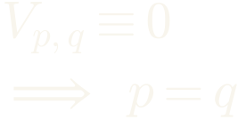Zero drift forces the two distributions to be equal

Definitions, and one rule

Half the work is refusing to assume the answer

Before anything can be proved, the objects have to exist inside the proof assistant. Here is the whole vocabulary. Each line is a definition in the repository, not a paraphrase of one.

Start with the kernel, which is the only thing in the method that decides whether two points count as close. This is the Laplace kernel: τ is a bandwidth you choose, and the value falls off with distance.

Two integrals against a distribution μ. The first adds up kernel weight, and the second adds up kernel-weighted displacement, meaning how far each sample sits from the probe point and in which direction.

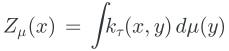
Z is called the normalizer and D the displacement numerator. They are the only two integrals in the entire argument. Everything that follows is built from them.

Divide one by the other and you get the mean shift: the weighted average direction from the probe point toward the distribution.

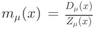
The drift field is one mean shift minus the other. Attraction toward the real data, repulsion from the model's own output.

And the hypothesis. Not "small", not "zero on average", not "zero where the data lives" — zero at every point of the space.

The same thing, in Lean

Nothing above is informal shorthand. This is how those definitions appear in the file, and the theorem quoted at the top of this page is stated in exactly these terms.

/-- Equation (9): the normalizing factor `Zₚ(x) = Eₚ[k(x,y)]`. -/
noncomputable def kernelNormalizer
    {E : Type u} [MeasurableSpace E]
    (k : E → E → ℝ) (p : Distribution E) (x : E) : ℝ :=
  ∫ y, k x y ∂p

/-- Equation (8): the normalized mean-shift field generated by one law. -/
noncomputable def meanShift
    {E : Type u} [MeasurableSpace E]
    [NormedAddCommGroup E] [NormedSpace ℝ E] [CompleteSpace E]
    (k : E → E → ℝ) (p : Distribution E) (x : E) : E :=
  (kernelNormalizer k p x)⁻¹ • ∫ y, k x y • (y - x) ∂p

/-- Equation (10): attraction by `p` minus repulsion by `q`. -/
noncomputable def meanShiftDrift
    {E : Type u} [MeasurableSpace E]
    [NormedAddCommGroup E] [NormedSpace ℝ E] [CompleteSpace E]
    (k : E → E → ℝ) : DriftingField E :=
  fun p q x => meanShift k p x - meanShift k q x

/-- The paper's notation `Vₚ,q(x) = 0, ∀x`. -/
def ZeroDrift
    {E : Type u} [MeasurableSpace E] [Zero E]
    (V : DriftingField E) (p q : Distribution E) : Prop :=
  ∀ x, V p q x = 0

The one rule that makes the exercise mean anything

A proof assistant will happily verify a proof of anything you have assumed. The danger in formalizing somebody else's argument is not making a mistake; it is quietly writing the conclusion into the setup and then deriving it back. A formal proof of a claim you assumed is a very expensive way of writing the claim down twice.

So the project puts every assumption in one file, and that file carries an explicit prohibition on the top of it:

Crucially, this file contains **no axiom** of either of the following forms:

* `ZeroDrift V p q → p = q`;
* `V p q = 0 → p = q` (pointwise, almost everywhere, or approximately).

Appendix C.1's ingredients are exposed separately, through the vanishing of
the coefficient minors `aᵢ bⱼ - aⱼ bᵢ`.  Turning those ingredients into an
identifiability theorem is deliberately left to downstream files.

A script enforces this on every run, and Section 08 shows how. For now the thing to hold on to is that the conclusion is never available as an ingredient, anywhere in the 53,709 lines.

Interactive

What the theorem is asking you to believe

Below is the drift field for two small distributions on a line. Blue points are the real data p; orange points are the model's output q. The curve is the field. The theorem says the only way to lay that curve flat on zero is to put the orange points exactly where the blue ones are. Drag them and see how close you can get.

The second view

Switch the panel to the defect and the curve changes to the quantity the proof is actually about. It is written H, it is built from the same two configurations, and it comes with a dashed envelope above it. Two features are worth noticing, because the entire argument runs on them: H stays under the envelope, and the envelope dies away from the data. Both facts are true for any pair of distributions, before anything at all is assumed about drift.

The first real move

Turning a fraction into a slope

The drift field is a ratio of two integrals minus another ratio of two integrals. Ratios are unpleasant to work with, and they hide the structure. The first move of the proof removes them.

Zero drift says the two mean shifts agree. Multiply out the denominators — legitimate, because Z is an integral of a strictly positive function and so is never zero — and the hypothesis becomes a statement with no division in it at all.

Now the observation that makes the rest possible. The displacement numerator D is not just some vector field. It is the slope of something. Consider this function of a distribution:

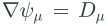
ψ is a potential and D is its gradient. Every point of the space now has a single number attached to it rather than an arrow, and numbers can be compared, maximized, and bounded in ways arrows cannot.

Why this survives at a single data point

There is a real obstacle buried in that identity, and the way it clears is the nicest small detail in the proof. The kernel contains a distance, and distance has a corner at zero: the function ‖x−y‖ is not differentiable when x sits exactly on y. If the identity broke there, the theorem would need distributions with no isolated points, and a great deal of generality would be lost.

It does not break. Write the potential as a profile applied to distance:

The derivative carries a factor of r, so it vanishes at the origin. A profile whose slope is zero at the corner is smooth enough to be differentiated through the corner: the offending kink gets multiplied by nothing. This is why the theorem needs no assumption about atoms.

/-- **`∇ψ_μ = D_μ`.**  For every finite measure, the displacement potential is
Fréchet differentiable with gradient the displacement field. -/
theorem hasFDerivAt_laplaceDisplacementPotential {τ : ℝ} (hτ : 0 < τ)
    (μ : Measure E) [IsFiniteMeasure μ] (x : E) :
    HasFDerivAt (laplaceDisplacementPotential τ μ)
      (innerSL ℝ (laplaceDisplacementField τ μ x)) x

With the potential in hand, define the ratio of the two normalizers. It is a ratio of positive numbers, so it is positive.

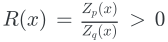
And the hypothesis becomes a statement about slopes:

Two landscapes whose slopes point the same way everywhere, differing only by a positive stretch factor that may vary from point to point. If that factor turned out to be the same number everywhere, the two distributions would be forced to agree. Proving it is constant is the whole remaining problem.

Interactive

One quantity, and three places it cannot hide

Here is the heart of it. Define a single number at each point, measuring how far the two landscapes are from being exact multiples of one another:

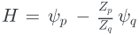
Call it the defect. If H is zero everywhere, the two potentials are proportional, and everything else follows. So the goal is now concrete: show H is identically zero.

The proof is by contradiction and it has the shape of a manhunt. Assume H is positive somewhere. Then it has to attain a largest value somewhere. Then check every place that largest value could sit — and find that none of them is possible. Select a step to see how each one closes.

/-- **The foliation defect vanishes identically under zero drift.**  The
maximum principle applied to both orders of the pair pins `H` between `0`
and `0`. -/
theorem laplaceFoliationDefect_eq_zero
    {τ : ℝ} (hτ : 0 < τ) (p q : Measure E)
    [IsProbabilityMeasure p] [IsProbabilityMeasure q]
    (hzero : ZeroDrift (meanShiftDrift (laplaceKernel τ)) p q) (x : E) :
    laplaceFoliationDefect τ p q x = 0 := by
  have h1 := laplaceFoliationDefect_nonpos hτ p q hzero x
  have h2 := laplaceFoliationDefect_nonpos hτ q p
    (zeroDrift_meanShiftDrift_symm hzero) x
  rw [laplaceFoliationDefect_swap hτ p q x] at h2
  have hR := laplaceNormalizerRatio_pos hτ q p x
  by_contra hne
  have hlt : laplaceFoliationDefect τ p q x < 0 := lt_of_le_of_ne h1 hne
  nlinarith [mul_pos hR (neg_pos.mpr hlt)]

From proportional to equal

Three steps that are each easier than they sound

One: the stretch factor is constant

A vanishing defect says the ratio of normalizers equals the ratio of potentials. That is now a quotient of two differentiable functions with a strictly positive denominator, so it can be differentiated by the ordinary quotient rule — and when you do, the alignment identity from Section 04 cancels the numerator exactly.

A function on a connected space with derivative zero everywhere is constant. Euclidean space is connected, so one constant covers all of it.

Two: smoothing cannot lose information

The normalizer Z is the distribution seen through a blur: every sample smeared by the kernel and added up. The step needed is that the blur is reversible in principle — two different distributions cannot blur to the same picture. Then equal normalizers force p to be c times q as measures.

The standard route to this fact goes through Fourier analysis and, in higher dimensions, through Bessel functions that are unpleasant to handle formally. The project takes a different road. The Laplace kernel can be written as a positive mixture of Gaussians, and Gaussians are already known not to lose information. The identity that does it comes from a classical integral:

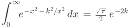
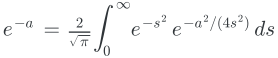
Read the second line from right to left: the exponential on the left is an average of Gaussians, all with positive weight. A positive mixture of things that each have a positive Fourier transform has a positive Fourier transform, which is never zero, which is exactly the condition for the blur to be reversible. No Bessel function appears anywhere.

Three: the constant is one

This last step is arithmetic. Both distributions have total mass one, because both are probability measures. If one equals c times the other, then 1 = c · 1.

  have hpScaled : p = (ENNReal.ofReal c) • q :=
    hL4 p ((ENNReal.ofReal c) • q) inferInstance hscaledFinite hZscaled
  have hmass : ENNReal.ofReal c = 1 := by
    have hpMass : p Set.univ = 1 := measure_univ
    rw [hpScaled, Measure.smul_apply, smul_eq_mul, measure_univ, mul_one] at hpMass
    exact hpMass
  rw [hpScaled, hmass, one_smul]

Interactive

Which file supplies which fact

The chain from the definitions to the theorem, as it exists on disk. Select any file to see what it contributes and what it needs from below it.

Ninety-six modules is more than this map shows. The omitted ones are earlier routes to the same destination — the one-dimensional case, the Gaussian kernel, the radial families in two and three dimensions, the absolute-continuity route — each closed before the general argument existed, and each now a special case of it. They are kept because a research record that deletes its own scaffolding is not a record.

The part people skip

How the project stops itself from cheating

A machine-checked proof is only as good as the question it was asked. There are three well-known ways to produce a green checkmark that means nothing, and the repository has a script guarding against each.

1. Leaving a hole and forgetting

   Lean lets you write sorry where a proof should be. Everything downstream still compiles. The audit scans every file, with comments stripped first so that the word can be discussed in prose, and fails the build if it appears in code.

   0 found across 96 modules

2. Adding an assumption quietly

   New assumptions are the easy way past a hard step. The audit holds a list of every assumption the project is allowed to make, by name, and compares it against what is actually declared. Adding one, renaming one, or moving one into another file fails the build.

   21 allowed 15 from the paper, 1 standard, 5 conditional

3. Editing the assumptions file

   A list of allowed names does not stop somebody changing what an allowed name says. So the file itself is fingerprinted, and the fingerprint is stored separately. Any edit at all, including one that keeps every name identical, fails the build until the change is deliberately re-approved.

   SHA-256 pinned in .trusted/

if ($code -match '(?m)\b(sorryAx|sorry|admit)\b') {
  $errors.Add("$relative contains a forbidden proof escape: sorry/admit/sorryAx.")
}
...
$actualHash = (Get-FileHash -LiteralPath $paperAxioms -Algorithm SHA256).Hash
if ($actualHash -ne $expectedHash) {
  $errors.Add(
    'Paperaxioms.lean changed without an approved trust-boundary update. ' +
    "Expected $expectedHash but found $actualHash."
  )
}

And then the question that settles it

Lean can be asked what a finished theorem actually rests on. The answer is not a summary or a claim; it is computed from the proof term. Asked about the headline result, it returns the three axioms that come with the logic itself — that propositions with the same truth value are equal, that you may choose an element from a nonempty collection, and that quotients respect the relation they are built from.

$ lake env lean AxCheck.lean

'DriftingIdentifiability.laplaceZeroDrift_identifies_euclidean' depends on axioms:
  [propext, Classical.choice, Quot.sound]
'DriftingIdentifiability.laplaceZeroDrift_identifies_rn' depends on axioms:
  [propext, Classical.choice, Quot.sound]

Two dead ends, and why they matter

The obvious proof does not exist

The argument in Section 05 is strange. A maximum principle, a backward flow, a symmetry swap — that is a lot of machinery for a statement about two distributions. There is a much more natural route, and the reason it is not on this page is that somebody checked and it is false.

In one dimension the proof is short, and it turns on a single inequality: the map that sends a point to that point plus its mean shift never runs backwards. Monotone maps are easy to invert, inverting the map identifies the distribution, and the theorem falls out. Every instinct says to prove the same inequality in higher dimensions and reuse the argument.

It fails, and not by a little. A family of two-point distributions drives the relevant quantity to minus infinity as the two points separate:

Refuted Predicted values −0.625, −1.875, −6.250, −18.750 as the separation grows; measured −0.624, −1.874, −6.249, −18.749. The failure direction is transverse to the drift, which is why nobody notices it by looking at one-dimensional slices.

The natural repair is to stop asking for the inequality in every direction and ask only along the drift itself, which is all a flow-line argument would consume. A three-point family kills that too, again without bound:

Refuted Also matched to three decimals against the closed form. Together these say something sharp: in two or more dimensions there is no pointwise sign control on the drift Jacobian, in any direction at all.

Both counterexamples were found numerically first, by scanning for violations and then optimizing adversarially to see whether the violation was bounded. It was not. Only afterward were the closed forms derived and checked against the measurements. That order matters: the scan was set up to look for the refutation, and it found one.