Independent research · 2026
Drifting without
an encoder
Drifting judges a generator by comparing its samples against real ones, so it needs to know when two images count as alike. That usually means borrowing a pretrained network. This model answers the question with its own learned features, and produces an image in a single network call.
- 13.17
- Clean FID, 50k samples
- 1
- Network call per image
- 0
- Pretrained networks used
- 6.4×
- Better than the starting point
In plain terms
Most image generators work by starting from static and removing a little of it at a time, often taking hundreds of passes to produce one picture. This project trains one that does the whole journey in a single pass. The training method it builds on, called drifting, compares a batch of real photographs against a batch the model has just produced and works out a correction that nudges the model's output toward the real data. To make that comparison it has to decide when two pictures count as similar, and the usual answer is to measure distance inside a network somebody else already trained — which quietly brings along that network's training data and its blind spots. Here the model judges similarity using its own internal features, learned from scratch alongside everything else, so no borrowed network appears anywhere in training. The generator is a 37.7-million-parameter transformer trained on CIFAR-10, a standard collection of 50,000 small photographs, and picture quality is scored with FID, where lower is better. It finished at 13.17, starting from 83.65.
Every drifting model has to decide when two images are similar. Where should that judgement come from?
Drifting trains a generator without a discriminator and without computing probabilities. It looks at where real samples sit, looks at where generated samples sit, and builds a field that points from one cloud toward the other. Push that field to zero and the two distributions meet. The approach is unusually stable for what it does, because there is no second network being trained against the first.
All of it rests on distance. Each sample is weighted by how far it sits from a probe point, so distance carries the entire notion of similarity. In pixel space it carries it badly. Two photographs of one subject, shifted a few pixels, land far apart. Two unrelated pictures that share a background colour land close together. A field built on those distances chases the wrong thing.
The standard repair is to measure distances inside a pretrained encoder, where nearby points tend to share content. It works, and it brings a dependency with it. The generator inherits that network's training data and its blind spots. Claims about training without supervision get harder to state. And since the usual quality scores are computed inside pretrained networks too, the objective and the metric end up sharing machinery.
This project removes the encoder from training. Distances are measured either directly in pixels or inside the generator's own hidden features, which are learned from scratch alongside everything else. What follows is the whole method, the parts you can play with, and an account of what the result does and does not settle.
A second thread runs alongside. Diffusion models generate by removing a little noise at a time, often hundreds of passes for one image. A one-step model does the journey in a single pass, which is hundreds of times cheaper, and much harder to train, because the network cannot correct itself along the way. Mean Flow showed how: teach the network that one big jump has to agree with the many small steps it replaces. That is the foundation this model builds on.
Euler Mean Flow
Teaching one jump to agree with many
Start by mixing an image with noise. Pick a number t between 0 and 1 and blend:

x is a real image and ε is random noise of the same shape. At t = 0 you have the clean image, at t = 1 pure noise, and in between a half ruined picture.
The network reads one of those mixtures and predicts the clean image behind it. It takes two extra numbers:

θ are the weights, t is the current noise level, and r is the level being jumped to, so h is the distance travelled. Half of every batch trains at h = 0, which is ordinary supervised denoising and anchors everything else.
The consistency rule
A network that only practised short jumps would still need many calls to generate. So the other half of the batch enforces agreement between scales. First measure how far the network's own answer moves when the jump shrinks slightly:

δ is a small step, 0.001 in this run. This is a finite difference: it approximates the rate at which the prediction changes as the jump size varies.
Scale that quantity and add it to the clean image to form the target:


c weights the correction by how long the jump is and how close its landing point is to clean data. The floor of 0.1 keeps it finite as r approaches zero. sg is a stop gradient: the value is used as a fixed number and the network cannot adjust how it was computed. Without that block the network could satisfy the rule by making all of its answers equally uninformative.
The loss is then ordinary squared error against that target:

Once trained, generating is a single call at the largest available jump. Noise goes in, an image comes out.

Where training looks, and where sampling happens
Sampling always asks for the far corner of the triangle, t = 1 and h = 1. Training almost never goes there. Drag the thresholds and watch how little of the training distribution sits near the point every image is drawn from.
This is a property of the recipe, not of any particular run. Feeding the corner more heavily was tested and made results worse: those rows come out of the short interval examples that keep the objective well posed.
The drifting correction
A field that points at what the generator is missing
The foundation learns the general shape of the data and tends to leave gaps, producing plausible images while quietly skipping certain kinds altogether. The correction pushes it toward whatever it is missing.
Weight every sample by how close it is, using a softmax over distances:
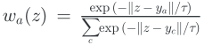
τ is the bandwidth. It sets how quickly influence falls away with distance, so nearby samples take most of the weight and distant ones take almost none.
Then subtract the weighted average of generated samples from the weighted average of real ones:

The result is an arrow at every point, pointing away from wherever the generator piled up too much and toward wherever the real data actually sits. Those distance weights supply the entire notion of similarity, which is why the method needs no pretrained encoder.
A single bandwidth sees only one scale, so several run at once and their errors are added:
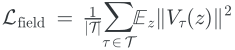
Squaring each bandwidth separately before summing matters. Adding the arrows together first would let two wrong fields cancel each other out.
Run it
Blue is real data. Orange is what the generator produced. Every orange point moves along the field. Press run and watch the energy fall and the coverage climb.
The simulation runs the field as a particle update so the mechanism is visible. In the trained model the same quantity becomes a gradient on the network's weights, capped so it can never outweigh the main objective.
Two more pieces
A frequency check, and a cap on everything
Comparing distributions by their frequencies
A second correction compares the two distributions through their characteristic functions:

ω is a random frequency drawn from a distribution ρ, with p the real distribution and q the generated one. The exponential is a wave pattern, so the quantity asks whether both sets of samples respond to the same waves the same way on average. If ρ covers all frequencies, this reaches zero exactly when the two distributions are identical, which gives this term a clean guarantee the field alone does not have.
That guarantee is about the ideal expectation. A finite bank of frequencies does not determine a distribution, so the bank is refreshed during training and no single frozen bank is ever the identifying object.
Why nothing is allowed to dominate
Neither correction serves as the loss. Each produces its own gradient, which is shrunk before it is added:

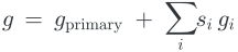
A correction already under its cap passes through untouched, and a larger one is scaled down until it fits. The caps are 0.15, 0.10 and 0.10.
The experiment lives in one line of that list. Two of the three corrections are the same field computed in two different places, once directly on pixels and once inside the model's own features. Nothing changes but the space the distances are measured in. On real images the feature version helped and the pixel version hurt, badly enough that a gate on its own field energy stopped two runs early.
Averaging the checkpoints
Training never settles on one setting of the weights. Every update comes from a small random batch, so the weights keep circling a good region without stopping inside it, and any single checkpoint is a slightly random pick from that region. Save the weights periodically and average them once training ends:
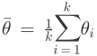
It is the weights themselves being averaged, not the images they produce. Much of the jitter is random and cancels. Generation then runs with the averaged weights.

There is a limit. Average in checkpoints from too early and you mix in weights from when the model was worse, and the result degrades with them. A moderate window works and past some width the benefit disappears. The final model averages 47.
Interactive
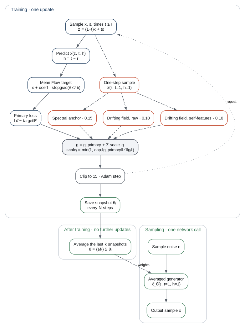
One training update, end to end
Select any stage to see what it computes and why it is there. Blue is the primary objective, orange the capped corrections, green the averaging and sampling path.
Training, one update
In parallel, from a one-step sample
After training, then sampling
See the whole thing as one diagram
CIFAR-10, unconditional
What was trained, and the three repairs that made it work
CIFAR-10 is 50,000 photographs at 32 by 32 pixels in ten categories. The generator is a 37.7M parameter transformer that reads each image as a grid of patches. It is trained unconditionally, so it is never told which category to produce, and evaluated with FID against the training reference on 50,000 samples.
Before anything else worked, the objective had to be made trainable. Three changes mattered more than every architectural choice combined, and all three were repairs to something already broken rather than new ideas.
-
Draw the times evenly
The original distribution was skewed and rarely visited the setting used for generation. Drawing two uniform endpoints and sorting them fixed the coverage of the triangle.
-
Cap the weight on very noisy examples
The loss weighted extremely noisy rows so heavily that a handful of them set the direction of nearly every update. Flooring that weight stopped it.
-
Raise the limit on update size
Almost every update was hitting the old clip, which flattened the learning rate schedule into decoration. Matching the clip to the gradients actually observed restored it.
Those three together moved FID from 83.65 to 18.92, more than every later change combined.
Interactive
Four stages, one seed, no cherry picking
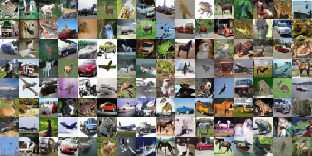
Every grid is the first 128 draws from the same random seed, recorded in the run metadata, so the panels are directly comparable. Select a stage, then click any tile to follow that exact sample through all four.
Same noise, four stages
Sample 0
The seed is fixed, so this is one image being generated from the same noise vector by four different sets of weights.
| Stage | FID | KID | What changed |
|---|---|---|---|
| Starting point | 83.65 | Not recorded | The objective as originally written |
| Repaired objective | 18.92 | 0.01193 | Time sampling, loss weighting, gradient clip |
| Drifting correction | 14.98 | 0.00903 | The field read in the model's own features |
| Checkpoint averaging | 13.17 | 0.00791 | Averaged 47 saved checkpoints, no further training |
The improvement arrived almost entirely as better coverage. The model produced a wider variety of images while the quality of any individual picture stayed roughly where it was, which is what the drifting correction is designed to do. Precision held near 0.73 throughout while recall climbed from 0.076 to 0.552.
The whole thing in one pass
From noise to an image
Training, one step
Draw a real image, some noise, and two times. Blend the image and noise to make the input. The network predicts the clean image, and the target it is scored against is that image plus a correction forcing long jumps to agree with short ones. That gives the first gradient.
Separately, generate a batch from noise, one call each. Compare them against real samples twice, once with the drifting field and once with the frequency anchor. Each comparison gives its own gradient. Shrink those so neither can outweigh the first, add everything, take a single optimiser step. Every few thousand steps, save a copy of the weights. Repeat several hundred thousand times.
After training
Take the last several saved copies and average them into one set of weights. Nothing is trained further. This step is arithmetic on files already on disk.
Generating
Draw a vector of random noise the same shape as an image. Pass it through the averaged network once, asking for the largest jump it knows how to make. What comes out is the image. There is no second pass, no noise schedule, and no refinement stage.
Read this before quoting the number
What the result settles, and what it leaves open
Where similarity is judged matters
The same field, computed on raw pixels, made results worse. Computed inside the model's own features, it made them better. In the one contrast that varies only the self-feature term, FID moved 22.54 to 16.10. That gap is the finding.
The metric still uses a pretrained network
FID runs inside Inception. Training no longer depends on a pretrained model, but the measurement does, so the dependency has moved rather than disappeared.
Self-judgement is circular
A fixed external encoder cannot drift. Features learned alongside the generator can, and nothing in the objective forces them to stay meaningful. The caps limit how much damage that could do without ruling it out.
One correction was never isolated
Every run had the frequency based correction switched on, so its own contribution has not been measured. One additional run would settle it.
A tail the score cannot see
One configuration produced a small share of wildly out of range samples while its FID still looked healthy, because FID is computed after images are clipped. Recording the largest pixel value alongside FID would catch it for nothing.
The ceiling is architecture and compute
Every structural change tried made the result worse, and more training of the same kind did not help. The remaining headroom sits outside these weights.
References
Liu, Y. et al. Euler Mean Flow. arXiv:2602.02571
Deng, Z., Li, X., Li, Y., Du, C. and He, K. Generative Modeling via Drifting. arXiv:2602.04770
Acknowledgement
The experimental code, the analysis, and this write-up were produced with the assistance of Claude, an AI system made by Anthropic. Every number reported here is an output of the code in the repository, measured through the same sealed evaluation path each time.
Continue exploring