Independent research · 2024
Forecasting
U.S. GDP
Four models, 64 years of quarterly data, and a 26-quarter test period that happens to contain the pandemic. The random forest posts the lowest error. Most of that error comes from two quarters, and what is left says something different about the result than the ranking does.
- 257
- Quarters, 1960 to 2024
- 4
- Model families compared
- 288
- Best holdout MAE, $bn
- 42%
- Of that error, from 2 quarters
In plain terms
Gross domestic product is the standard headline measure of how much an economy produced in a given period, and forecasts of it feed into decisions that get made before the official figure arrives. It is also, by definition, the sum of four things: what households consume, what businesses invest, what government spends, and what the country sells abroad minus what it buys. This project asks whether those four components, tracked quarterly since 1960, carry enough structure to predict the next move in GDP. It pulls five series from FRED, the Federal Reserve's public data service, runs the standard checks that decide which models are even applicable, and then puts four of them on the same 26-quarter test period: two classical time-series models from econometrics and two general-purpose machine learning models. It was written in Python with pandas, statsmodels and scikit-learn. The random forest records the lowest error, which is the result the original write-up reported — and the sections below take that number apart to show what it is and is not measuring, because the test period contains the sharpest two quarters in the history of the series.
Four numbers add up to GDP. Do they also predict it?
GDP is not an estimate of anything mysterious. It is an accounting identity: consumption plus investment plus government spending plus net exports. The four components are published alongside it, on the same quarterly schedule, from the same national accounts.
So the identity itself is not a forecast — it holds exactly, after the fact, and knowing three components tells you the fourth only once all four are measured. The question is whether the recent history of those components carries information about where the total goes next.
One decision shapes everything downstream. The target here is not the level of GDP but the quarterly change in it. Levels grow relentlessly, so predicting a level is mostly predicting a trend and any model looks impressive. Predicting the change is the part that is genuinely hard.
The test period runs from 2017 Q4 to 2024 Q1, the last 26 quarters of the dataset, held out in chronological order. That window includes 2020, which turns out to matter more than any modelling choice made anywhere else in the project.

The five series pulled from FRED are GDP itself, personal consumption expenditures, gross private domestic investment, net exports, and total government expenditure. Everything is nominal and quarterly, inner-joined into 257 aligned rows from 1960 Q1 to 2024 Q1.
Diagnostics before modelling
Two things are wrong with the raw series
Most time-series models will not work on data that trends, and no model gives interpretable coefficients when the inputs move together. Both problems are present here, and only one of them gets fixed.
The series are not stationary
An augmented Dickey–Fuller test asks whether a series has a stable mean and variance. Small p-values mean stationary. Every raw series comes back at essentially 1.0 — as nonstationary as the test can report, which is what you would expect of anything that grows for sixty years.
The fix is differencing: model the change from one quarter to the next instead of the level itself.

After one difference every series clears the test comfortably. That is also the moment the target quietly becomes the quarterly change, and every error figure on this page is in those units.
The predictors are nearly the same variable
A variance inflation factor measures how much of one predictor is explained by the others. Anything above 5 is usually called a problem. Consumption comes back at 170.
Switch the panel between the raw and differenced data to see what differencing fixes and what it leaves alone.
Stationarity ADF p-value, lower is stationary
Collinearity variance inflation factor, raw levels
Differencing does not appear here because the notebook measures inflation on the levels. The components share information by construction, and no transformation of them changes that.
This is what steers the model choice. With predictors that collinear, a linear model's coefficients stop meaning anything individually, even when its forecasts are fine. Tree models split on one variable at a time and do not have coefficients to corrupt, which is the stated reason the notebook reaches for a random forest.
One more check, and one thing it did not clear
A Granger causality test asks whether past values of one series improve a forecast of another. The notebook runs it per component and keeps a lag for each. Consumption is the awkward one: its best p-value sits just outside the usual 5% threshold at lag 6, and the notebook says so and keeps it anyway. That is a judgement call, and it is worth knowing it was made.
Two classical, two machine learning
What each one assumes
The four were not picked to be exotic. With 257 quarters there is not enough data to justify anything large, so the comparison is between models that write their assumptions down and models that make very few.
-
Vector autoregression
Classical · needs stationary input
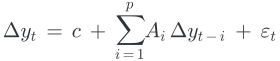
Every series is regressed on the recent past of every series, itself included. It captures how the components lead and lag one another, and it requires the differencing from the previous section to be valid at all. Fitted with up to 14 lags.
-
Vector error correction
Classical · works on the levels
Built for series that wander individually but stay tied together in the long run, which is exactly what an accounting identity produces. A Johansen test finds three such relationships, so the model is fitted on the raw levels with rank 3. It predicts levels, not changes, so its error is on a different scale from the other three and cannot be ranked against them.

-
Random forest
Machine learning · no assumptions about form
Many decision trees, each fitted to a resampled version of the data, averaged. It splits on one predictor at a time, so the collinearity from Section 02 does not hurt it, and it is hard to overfit by accident. 100 trees, fixed seed.
-
K nearest neighbours
Machine learning · no fitting at all
For a new quarter, find the most similar quarters in the training data and average what happened next. With five predictors and a thousand-odd observations the ratio is favourable. The notebook sweeps k from 1 to 9 and takes k = 2.
All four use the components measured in the same quarter as the GDP figure being predicted. In a live setting those numbers are not available yet, so this is closer to nowcasting than to genuine forecasting. Section 07 comes back to it.
Interactive
All four on the same 26 quarters
Every value here is read from the notebook's output. Switch between the quarterly change, which is what three of the models actually predict, and the accumulated level, which is what the change adds up to over six years.
| Model | Target | MAE | MAPE | Note |
|---|---|---|---|---|
| Random forest | Quarterly change | 287.97 | 44.31% | Lowest of the three comparable models |
| KNN, k = 2 | Quarterly change | 303.45 | 47.72% | Within 6% of the random forest |
| VAR, 14 lags | Quarterly change | 328.39 | 57.72% | The classical baseline |
| VECM, rank 3 | GDP level | 1,482.53 | — | Different target, not comparable |
MAPE divides by the actual value, and quarterly GDP changes pass through zero and go negative in this window. The percentages above are what the notebook printed, but they are not a stable way to compare these models and nothing on this page rests on them.
Interactive
Two quarters carry two fifths of it
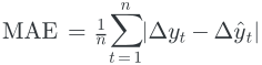
A mean absolute error is an average, and averages hide their own composition. Here is the same 287.97, broken out by quarter.
Each bar is one quarter's absolute miss. Use the switch to drop 2020 Q2 and Q3 — the collapse and the rebound — and watch what happens to the number and to the ranking.
What that means, and what it does not
In 2020 Q2 GDP fell by $1,793bn in a single quarter. The random forest predicted a fall of $162bn. One quarter later it rose by $1,734bn and the model predicted a rise of $234bn. Those two quarters alone contribute 41.8% of the model's total error over six years. The same is true of the other two: 41.1% for VAR, 41.0% for KNN.
None of this is a flaw in the models. Nothing in sixty years of data suggested a quarter like 2020 Q2 was possible, and a model that had somehow predicted it would have been wrong about everything else. The point is narrower: the headline MAE is largely a measurement of how badly each model handled one event, not of how well it tracks a normal quarter.
The ranking survives. Drop the two quarters and the random forest still leads, at 181.5 against 194.0 and 209.5. That is worth stating plainly, because it is the part of the original conclusion that holds up.
The comparison the notebook did not run
Better than what?
A model can be the best of four and still not be doing much. The way to find out is to put it against predictions that require no model at all.
| Prediction | MAE | Uses only past data | What it is |
|---|---|---|---|
| Always predict zero | 482.38 | Yes | Assume GDP does not move |
| Training average, +83.26 | 411.93 | Yes | The mean change over 1960 to 2017 |
| Last quarter's change | 367.98 | Yes | Assume the last move repeats |
| Random forest | 287.97 | Yes | The model from Section 03 |
| Best fixed number, +345.7 | 270.21 | No | Chosen after seeing the answers |
The first three are legitimate competitors: each could have been produced in 2017 with no knowledge of what followed. The random forest beats all of them, comfortably. That is a real result and the project earned it.
The last row is not a legitimate competitor. It is the single constant that would have minimised error over the test period, which nobody could have known in advance. It is in the table because of what it reveals: no constant could have scored better than 270, and the model scored 288. Whatever the random forest is doing, it is not beating the best a flat line could manage.
The models barely move
That result has a visible cause. Over the holdout, actual quarterly changes range from −$1,793bn to +$1,735bn, with a standard deviation of 536. The random forest's predictions range from −$162bn to +$297bn, standard deviation 97. The VAR is flatter still, at 45.
Each bar shows the range each series covers, on a common scale. The models occupy a narrow band near the middle: they have learned roughly how much GDP grows in a typical quarter and they mostly predict that, every quarter.
Which is a defensible thing for a model to do when the alternative is guessing at shocks. But it means the honest description of the result is not "the random forest forecasts GDP well". It is: the random forest learned the typical quarterly growth rate more precisely than a long-run average would give you, and it does not predict deviations from it.
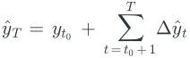
The accumulated view makes the same point. Add up the random forest's predicted changes across the holdout and you get a GDP level of $24.27tn at 2024 Q1 against an actual $28.26tn. Over six years the model recovers slightly more than half of the real rise, because the quarters it underestimates never get corrected — small errors in a differenced model compound when you put the levels back together.
Concretely
Four things, in order of how much they would matter
A fifth possibility, from the original write-up, was to smooth the 2020 to 2024 window before fitting. That would improve the metrics and I would not do it: the pandemic quarters are the honest part of this test, and removing them optimises for the score rather than the question.
Read this before quoting the number
What this is, and what it is not
A clean model comparison
Four families on identical data, an identical chronological split and an identical metric. The ranking holds with and without the pandemic quarters.
The machine learning models won
Both beat both classical models, and the notebook's reasoning for why — too few observations for VAR and VECM, collinearity that trees tolerate — is sound.
It is nowcasting, not forecasting
The predictors come from the same quarter as the target. Nothing here tells you what GDP will be next quarter, only what it was consistent with once the components were known.
Revised data, not real-time data
Every figure is the current revised estimate. Testing against numbers that were not available when the prediction would have been made is a known way to overstate accuracy.
One split, one number
No rolling validation, no confidence interval, no repeat runs. The 15-point gap between the random forest and KNN is well inside the range a different split could produce.
Not a GDP forecast
This is an archive of a July 2024 student project, and the data ends at 2024 Q1. It is a study of forecasting methods, not a current view on the economy.
Source
github.com/Dronmong/GDP-Forecast — the notebook. It needs a free FRED API key to run.
Forecasting US GDP using Machine Learning and Mathematics — the original write-up, published in Towards Data Science, July 2024.
Data
Federal Reserve Bank of St. Louis, FRED. Series GDP, PCE, GPDI, NETEXP and W068RCQ027SBEA, quarterly, nominal.
References
Hyndman & Athanasopoulos, and the two texts the notebook cites: Forecasting Time Series Data (Apress) for the classical models and An Introduction to Statistical Learning for the machine learning ones.
Acknowledgement
This page was written with the assistance of Claude, an AI system made by Anthropic. Every forecast value shown is read from the notebook's own output; the baseline and error-decomposition figures in Sections 05 and 06 were computed from those same values and are new to this page.
Continue exploring